How Erasure Coding Works

TL;DR

Erasure coding splits data into k data fragments, computes m parity fragments using linear algebra over Galois Fields (GF(2^8)), and distributes all k+m fragments across storage nodes. Any k of the k+m total fragments can reconstruct the original data. RS(10,4) achieves the same durability as triple replication at 1.4x storage overhead instead of 3x — at S3's scale (~280 exabytes), that delta is hundreds of millions of dollars per year in hardware.

The Problem: Replication Doesn't Scale

Traditional replication stores N identical copies. To survive 2 disk failures, you need 3 copies — 3x storage overhead. At exabyte scale, the math is brutal:

Strategy	Storage for 100 PB of data	Tolerated failures
3x replication	300 PB	2
RS(10,4)	140 PB	4
LRC(12,4,2)	150 PB	6

Erasure coding replaces copies with math. Instead of storing the same data 3 times, you compute parity fragments that encode the mathematical relationships between data fragments. Any sufficiently large subset of fragments — data or parity — can reconstruct the original.

Reed-Solomon Codes — The Workhorse

The dominant erasure code in production storage (S3, Azure Blob, HDFS, Ceph) is Reed-Solomon (RS). An RS(k, m) code splits an object into k data fragments and computes m parity fragments.

k = number of data fragments (data shards)
m = number of parity fragments (parity shards)
n = k + m = total fragments
Any k out of n fragments can reconstruct the original data
Tolerates up to m simultaneous fragment losses

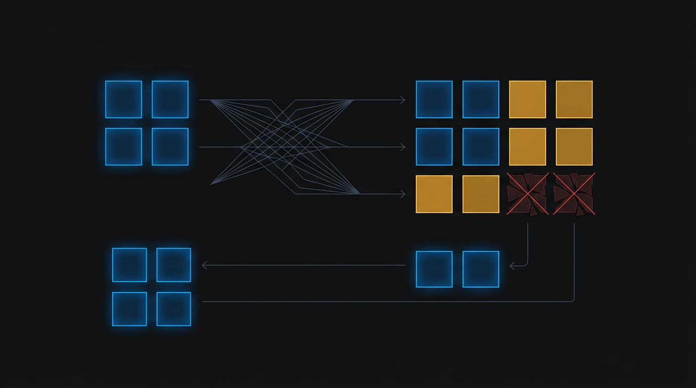
Reed-Solomon Erasure Coding — encoding and reconstruction flow

Galois Field Arithmetic — GF(2^8)

Reed-Solomon operates over a finite field, specifically GF(2^w) where w is typically 8. In GF(2^8), every element maps to exactly one byte (values 0–255), and every non-zero element has a multiplicative inverse — which is required for the decoding step.

Addition = XOR. No carries. a + b = a XOR b.

Multiplication = polynomial multiplication modulo an irreducible polynomial, typically x^8 + x^4 + x^3 + x^2 + 1 (0x11D).

In practice, multiplication uses pre-computed lookup tables:

// GF(2^8) multiply using log/exp tables (256 entries each)
uint8_t gf_mul(uint8_t a, uint8_t b) {
    if (a == 0 || b == 0) return 0;
    return exp_table[(log_table[a] + log_table[b]) % 255];
}

This converts multiplication to two table lookups, one addition, and one modulo — constant time, no branches, no timing side-channels.

Encoding: Generator Matrix Multiplication

The encoding process is a matrix multiplication in GF(2^8). Given k data fragments D = [D0, D1, ..., Dk-1], the encoder computes G x D = Output:

# Generator Matrix G (6x4, i.e. n x k)
G = [
  [ 1,   0,   0,   0  ],   # --> D0  (identity row)
  [ 0,   1,   0,   0  ],   # --> D1  (identity row)
  [ 0,   0,   1,   0  ],   # --> D2  (identity row)
  [ 0,   0,   0,   1  ],   # --> D3  (identity row)
  [ g00, g01, g02, g03 ],  # --> P0  (parity row)
  [ g10, g11, g12, g13 ],  # --> P1  (parity row)
]

# Output = G x [D0, D1, D2, D3]
# First 4 rows: identity matrix --> data passes through unchanged
# Last 2 rows: coding matrix   --> parity is computed

The top k rows are an identity matrix — this makes it a systematic code, meaning the original data appears unmodified in the output. The bottom m rows form the coding matrix. Each parity fragment is a linear combination of all data fragments:

P0 = gf_mul(g00, D0) ^ gf_mul(g01, D1) ^ gf_mul(g02, D2) ^ gf_mul(g03, D3)
P1 = gf_mul(g10, D0) ^ gf_mul(g11, D1) ^ gf_mul(g12, D2) ^ gf_mul(g13, D3)
# All operations in GF(2^8): ^ is XOR (addition), gf_mul is field multiplication

Choosing the Coding Matrix

Two standard constructions, each with different performance characteristics:

	Vandermonde	Cauchy
Construction	Row i: [α_i^0, α_i^1, ..., α_i^(k-1)]	Element (i,j) = 1/(x_i + y_j)
MDS proof	Vandermonde determinant = product of differences	Cauchy determinant formula
Encoding	GF multiply per element	Reduces to XOR-only after precomputation
Throughput	~400 MB/s (table lookup)	40+ GB/s (ISA-L, AVX-512)
Used by	Theoretical reference	Ceph, HDFS, ISA-L, most production systems

Most production implementations use Cauchy matrices because XOR-only encoding is 3–10x faster than table-based GF multiplication (Blomer et al., "An XOR-based Erasure-Resilient Coding Scheme," 1995).

Decoding: Matrix Inversion

When fragments are lost, reconstruction works by solving a linear system:

Select any k available fragments (data or parity)
Extract the corresponding k rows from the generator matrix G — call this submatrix G'
Compute G'^(-1) (inverse of the k×k submatrix) via Gaussian elimination over GF(2^8)
Multiply: [D0, D1, ..., Dk-1] = G'^(-1) × [selected fragments]

This works because G was constructed so that every k×k submatrix is invertible — the Maximum Distance Separable (MDS) property. The Vandermonde and Cauchy constructions both guarantee this.

Matrix inversion is O(k^3) in fragment count, but k is typically small (6–16), so inversion takes ~5 μs. The real cost is I/O: reading k fragments from k different storage nodes.

Concrete Example: RS(4,2)

# Data: 4 bytes, one per fragment
data = [0xAB, 0xCD, 0xEF, 0x01]

# Cauchy coding matrix (2×4 over GF(2^8)):
# [71   167  122  83 ]
# [198  29   51   240]

# Encoding (all arithmetic in GF(2^8)):
P0 = gf_mul(71, 0xAB) ^ gf_mul(167, 0xCD) ^ gf_mul(122, 0xEF) ^ gf_mul(83, 0x01)
P1 = gf_mul(198, 0xAB) ^ gf_mul(29, 0xCD) ^ gf_mul(51, 0xEF) ^ gf_mul(240, 0x01)

# Output: [D0=0xAB, D1=0xCD, D2=0xEF, D3=0x01, P0, P1]

# If D1 and P0 are lost, take rows for [D0, D2, D3, P1]:
# G' = [[1,0,0,0], [0,0,1,0], [0,0,0,1], [198,29,51,240]]
# Invert G', multiply by [D0, D2, D3, P1] → recover D1 and P0

How Production Systems Use Erasure Coding

S3

AWS hasn't published exact RS parameters, but the durability math constrains the design. S3 Standard promises 99.999999999% (11 nines) durability. Based on AWS re:Invent 2023 talks and public documentation:

Data is split across a minimum of 3 Availability Zones
Likely RS(11,6) or similar — ~17 total shards
Each shard stored on a different storage node, spread across AZs
Storage overhead: ~1.5x (vs 3x for triple replication)
S3 One Zone-IA uses replication within a single AZ (no cross-AZ erasure coding)

The key design choice: shards are distributed across AZs, not just across disks within one AZ. A full AZ outage (power, network, natural disaster) only loses a fraction of the total shards.

S3 Write Path (PUT Object)

Client sends PUT to the S3 frontend (HTTP endpoint behind a load balancer).
The frontend's placement engine selects which storage nodes across which AZs will hold the fragments — ensuring fragments land on different racks, different power domains, across at least 3 AZs.
The object body is split into k data shards, and m parity shards are computed using Reed-Solomon. Encoding uses ISA-L (SIMD-optimized) — ~25 μs/MB, not the bottleneck.
All n shards are written in parallel to their assigned storage nodes. Each shard is written with a CRC32c checksum and a shard index (0 through n-1). The frontend waits for a write quorum (e.g., at least 12 of 17 acknowledging) before returning 200 OK.
Metadata is written to the metadata service (DynamoDB-based): object key → shard locations, shard indices, version, checksums, ETag. The 200 OK only goes back after both the shard quorum AND the metadata write succeed.

Because it's a systematic code, shards 0 through k-1 ARE the original data (identity rows). No transformation needed for those — just chunking. Only the m parity shards require GF(2^8) computation.

S3 Read Path (GET Object)

Normal case — no failures:

Client sends GET. The frontend looks up the metadata to find shard locations and their indices.
Since it's a systematic code, the frontend reads just the k data shards — these ARE the original data. No decoding needed. Concatenate in order and stream back to the client.
In practice, S3 sends read requests to k+1 or k+2 shards (hedged reads), using the first k that respond to cut tail latency.

Degraded case — some shards unavailable:

If data shards are missing (node down, disk failed), the frontend reads any k available shards — mixing data and parity shards.
It extracts the corresponding k rows from the generator matrix (using each shard's index), inverts the submatrix (~5 μs), and decodes the original data.
The client has no idea a reconstruction happened — the S3 API returns the same response either way.
A background repair is triggered to replace the missing shard on a new storage node, restoring full fault tolerance.

How the System Knows Data from Parity

Every shard carries a shard index stored in the metadata service. When the frontend wrote shard #3 to Node B, it recorded that mapping. On read, when the first k responses arrive, the frontend checks their indices:

All indices in [0, k-1]? Fast path — these are identity rows. Concatenate in order, zero math.
Mix of data and parity indices? Slow path — pull those rows from the generator matrix, invert the k x k submatrix, multiply to recover the original k data fragments.

There's no guessing. The shard index is how the decoder knows which row of G each shard represents — without it, you wouldn't know which linear equation each shard encodes, and decoding would be impossible. The "systematic" property is purely a read-path optimization, not a mathematical requirement. Reed-Solomon treats all shards uniformly at the algebra level.

Azure Blob Storage

Azure publishes their design (Huang et al., "Erasure Coding in Windows Azure Storage," USENIX ATC 2012):

LRC(12,4,2): 12 data + 2 local parity + 2 global parity = 18 fragments
Storage overhead: 1.33x for the base RS portion
Survives any 6 simultaneous fragment losses

HDFS (Hadoop 3.0+)

Default RS(6,3): 6 data + 3 parity = 1.5x overhead
Previously used 3x replication — switching saved Yahoo ~47% storage (HDFS-7285)
Uses ISA-L for SIMD-accelerated encoding

Security & Data Integrity

Erasure coding provides no confidentiality — fragments are not encrypted. But it has critical integrity properties.

Silent Data Corruption (Bit Rot)

Any single bit flip in a fragment will produce incorrect reconstruction. The defense is layered:

Layer	Mechanism	Detection Rate
Fragment-level	CRC32c per shard	99.99999998% of random errors
Object-level	Content-MD5 / SHA-256	Catches corrupted reconstructions
Background	Continuous scrubbing	Reads all fragments, re-encodes, verifies

S3's scrubbing process runs continuously, checking a fraction of objects each hour. Typical enterprise scrub intervals: weekly to monthly.

Erasure vs Error Correction — A Critical Distinction

RS codes in storage are used as erasure codes, not error-correcting codes:

Erasure: The system knows which fragments are missing (the disk is dead, the node is unreachable). Positions are known.
Error: The system does not know which fragments are corrupted — it must detect AND correct.

An RS(k, m) code can correct up to m erasures but only ⌊m/2⌋ errors. In storage, checksums convert errors into erasures: detect corruption → mark fragment as missing → reconstruct. This doubles the effective fault tolerance.

Scaling & Performance — With Numbers

Encoding Throughput

Encoding is the critical hot path — every write must encode before acknowledging:

Implementation	Throughput	CPU	Method
Naive GF multiply (table lookup)	~400 MB/s	Single core x86	Lookup table per byte
ISA-L (Intel)	40+ GB/s	Xeon, AVX-512	SIMD vectorized Cauchy XOR
Ceph Jerasure	~2 GB/s	Single core	Optimized Cauchy
Go `klauspost/reedsolomon`	~10 GB/s	AVX2, 8 cores	Hand-written assembly kernels

Why ISA-L is fast: Cauchy matrices reduce all GF(2^8) multiplications to XOR operations. XOR is SIMD-friendly — AVX-512 processes 64 bytes per instruction. For RS(10,4), encoding one stripe requires ~40 XOR passes on 512-bit vectors:

Encoding rate = (512 bits/XOR * effective_clock) / (XOR_passes * bits_per_chunk)
             ~= 40+ GB/s on a single Xeon core with AVX-512

ISA-L also uses cache-friendly data layouts (striping across cache lines) to avoid L1/L2 thrashing. Source: https://github.com/intel/isa-l

Decoding (Reconstruction) Latency

Step	Latency
Matrix inversion (k=10)	~5 μs (one-time per reconstruction)
Fragment I/O (read k fragments, parallel SSD reads)	100–500 μs per fragment
GF decode (same throughput as encode)	~25 μs per MB
Network transfer (cross-node)	1–10 ms per fragment
Total degraded read	~2–5x normal read latency

AWS re:Invent sessions report p99 GET latency increases by ~30% during AZ maintenance events that require reconstruction.

The Tail Latency Problem: Degraded Reads

When a fragment is unavailable, the system must fan out to k nodes instead of reading 1 (as described in the S3 read path above). This is strictly slower than reading from a replica. The hedged read strategy mitigates this even in the normal case: send requests to k+1 or k+2 fragments, use the first k that respond. This trades bandwidth for latency — and the shard index on each response tells the decoder exactly which rows of G it's working with.

<details> <summary>Hedged reads — the math</summary>

If each fragment read has latency drawn from a distribution with p99 = 10ms, reading k=10 fragments in parallel means you're waiting for the slowest of 10 reads (order statistic). The expected max of 10 draws from a 10ms-p99 distribution is significantly higher than 10ms.

By reading k+2=12 fragments and using the first 10, you're waiting for the 10th order statistic of 12 — which is much closer to the median. Dean & Barroso, "The Tail at Scale" (CACM 2013), showed this technique reduces tail latency by 40–60% in practice.

</details>

Failure Modes — Concrete Scenarios

1. Reconstruction Storm After Node Failure

When a storage node dies, ALL objects that had a fragment on that node must be reconstructed. For a 100 TB node with RS(10,4):

~10M objects affected (at 10 MB average)
Each reconstruction reads 10 fragments from 10 different nodes
Total cross-node I/O: ~1 PB
At 10 Gbps per node: ~22 hours to reconstruct

During this window, fault tolerance is reduced. If another node fails before reconstruction completes, and both failed nodes held fragments of the same object, that object's tolerance drops from m=4 to m=2. Correlated failures (shared power supply, rack switch failure) can exploit this window.

2. Correlated Failures

RS(k, m) assumes independent failures. Reality disagrees:

Disks from the same manufacturing batch (same firmware bug)
Nodes in the same rack (shared power, shared ToR switch)
Nodes in the same AZ (shared infrastructure)

A batch of 1000 disks with a firmware bug that triggers after 40,000 power-on hours could lose 50+ disks simultaneously. RS(10,4) doesn't survive 50 simultaneous losses.

Mitigation: Fragment placement policies. HDFS's rack-awareness ensures fragments spread across racks. S3 spreads across AZs. Azure's LRC adds local parity groups.

3. Metadata Corruption

The mapping "object X → fragments [f0@node1, f1@node7, f2@node15, ...]" is stored in a metadata database. If this mapping is lost or corrupted, the system cannot locate the fragments for reconstruction.

You have all the fragments but can't find them. This is operationally worse than losing the data. S3 stores this mapping in a DynamoDB-based metadata service with its own replication — the metadata layer is the most critical component.

4. Silent Corruption Without Scrubbing

If fragment A is silently corrupted and the corruption isn't detected before fragment B is also lost, reconstruction produces garbage data silently. The reconstructed data may pass fragment-level CRC checks (because the CRC was computed on the corrupted fragment), but the content is wrong.

Detection: End-to-end checksums at the object level (not fragment level). S3 computes Content-MD5 and Content-SHA256 at the object level. Early HDFS-EC deployments only had fragment-level checksums — this was a known gap (fixed in HDFS-14768).

Trade-offs & Alternatives

	3x Replication	RS(10,4)	LRC(12,4,2)	RAID-6 (local)
Storage overhead	3.0x	1.4x	1.5x	1.17x (6+2)
Write latency	1 RTT (parallel)	Encode + 14 writes	Encode + 18 writes	Encode + 8 local
Read latency (normal)	1 read (full copy on replica)	k=10 parallel reads, no decode (systematic)	k=12 parallel reads, no decode (systematic)	1 stripe read
Read latency (degraded)	1 read (another replica)	k=10 reads + decode (data + parity mix)	~6 reads from local group + decode	Full stripe + decode
Reconstruction traffic	1 full copy (low fan-out)	k reads from k nodes (high fan-out)	~6 reads (local group)	Local to the node
Max tolerated failures	2	m=4	6 total	2
Best for	Write-heavy, small objects	Large objects, archival	Cloud-scale (>100 PB)	Single-server

Local Reconstruction Codes (LRC)

Standard RS requires reading k fragments from k different nodes for ANY reconstruction — even a single fragment loss. LRC (Huang et al., USENIX ATC 2012) organizes fragments into local groups, each with its own local parity:

Global:        [D0 D1 D2 D3 D4 D5 D6 D7 D8 D9 D10 D11 | GP0 GP1]
                                                           ^-- global parity

Local group 1: [D0  D1  D2  D3  D4  D5  | LP0]  <-- local parity
Local group 2: [D6  D7  D8  D9  D10 D11 | LP1]  <-- local parity

If D3 is lost, only 5 fragments from local group 1 are needed (not all 12). This cuts reconstruction I/O by ~50%.

When to Use What

Scenario	Recommendation	Why
Hot data, write-heavy, <1 MB objects	3x replication	Encoding overhead dominates for small objects
Warm/cold data, >1 MB objects	RS(10,4) or RS(6,3)	Storage savings justify encoding cost
Cloud-scale (>100 PB)	LRC	RS reconstruction I/O would saturate the network
Single server	RAID-5/6 (local RS)	No network overhead; mdraid or ZFS handles it
Archival (11+ nines)	Deep RS(17+) + cross-AZ	S3 Glacier-like configurations

Production War Stories

The Config Everyone Gets Wrong: Chunk Size

RS codes operate on stripes — each stripe is k chunks of size S. The chunk size dramatically affects performance:

Too small (64 KB): Many stripes per object → more metadata → more I/O. HDFS-EC originally defaulted to 64 KB and users reported 4x latency degradation for small random reads (HDFS-10301).
Too large (64 MB): A 1 KB file with RS(10,4) would occupy 640 MB of space. Wasted.
Sweet spot: 1–4 MB is typical for object storage. HDFS settled on 1 MB after benchmarking (HDFS-14768).

The Monitoring Gap: Reconstruction Queue Depth

Most teams monitor disk failures. Few monitor reconstruction queue depth — how many objects are waiting to be reconstructed.

Time to vulnerability = (queue_depth * avg_reconstruction_time) / parallelism

If this queue grows faster than the system can drain it, you're in a race: another failure during the window means reduced fault tolerance for objects still in the queue. Monitor: reconstruction backlog (objects pending), reconstruction throughput (objects/sec), and time-to-full-recovery.

The Version Upgrade That Broke Everything

HDFS 3.0 introduced erasure coding. The initial implementation (HDFS-7285) used a Java-based RS codec that was 10x slower than ISA-L. Hadoop deployments that upgraded to 3.0 saw write throughput collapse because encoding was CPU-bound in the JVM. The fix: ISA-L native codec (HDFS-7320) — but operators had to explicitly enable it and install the native library. It wasn't the default.

References

Reed & Solomon, "Polynomial Codes Over Certain Finite Fields," J. SIAM, 1960 — the original paper
Huang et al., "Erasure Coding in Windows Azure Storage," USENIX ATC, 2012 — LRC design and production deployment at Azure
Muralidhar et al., "f4: Facebook's Warm BLOB Storage System," OSDI, 2014 — RS at Facebook scale for photo/video storage
Plank, "Erasure Codes for Storage Systems: A Brief Primer," ;login: USENIX Magazine, 2013
Dean & Barroso, "The Tail at Scale," CACM, 2013 — hedged reads and tail latency mitigation
ISA-L source: https://github.com/intel/isa-l — Intel's SIMD-optimized RS implementation
HDFS-7285: https://issues.apache.org/jira/browse/HDFS-7285 — HDFS erasure coding feature JIRA